Transmission Expansion Planning Problem
The primary purpose of the electrical grid is to safely and reliably transport electricity from electrical power generation units to consumers. To this end, electrical grid infrastructure’s primary components consists of several types of power generating units, called “generators,” which use steam, water, wind, solar, fossil fuels, and nuclear energy to create power, in addition to devices which are used for appropriately reducing or increasing voltage as electricity travels to its end destination, lines for transporting the generated energy, and energy storage facilities that allow excess generated energy to be used at a later time. Designation of resources to further developement of grid infrastruture technology is based off of projected demand for energy, whereby improvements are made to existing grid configurations in order to ensure the reliability and safety of the transportation of energy under predicted increased demand.
Common problems which seek to aid in planning of grid improvements often focus on increasing transmission and generation aspects of existing grid infrastructure. In which case, a mathematical model can be developed to assess the best possible configuration resulting in an adequate number of either generators or lines to be installed that provides least costs and proper coverage. However, it is generally observed that such exploration of generator and line installation configurations are conducted separately so as to avoid an overly complicated mathematical model. Particularly, for planning related to line expansion, a so-called transmission expansion planning problem (TEP) is solved, whereas a generation expansion planning problem is to be solved for planning related to generation. In this blog post, the former is explored, and a primary focus is placed on an application of TEP which utilizes a moderately-sized and well-known test system.
Transmission Expansion Planning Model
In an abstract sense, TEP is modeled as an undirected graph $(V,E)$ with edge set $E$ and set of vertices $V$ corresponding to lines and buses within the electrical network, respectively. As TEP’s goal is to determine how many, and which lines from a set of candidate lines should be installed to meet predicted demand, the edge set $E$ will be partitioned so as to distinguish edges that can potentially be installed from those which are already installed. Table 1 below more precisely describes parameters, variables, and sets which are used to formalize the transmission of electricity across grid instances in the context of TEP.
| Symbol | Description |
| Sets | |
| $\mathcal{G}$ | Set of generators |
| $\mathcal{E}^{\nu}$ | Set of new lines |
| $\mathcal{E}^{\epsilon}$ | Set of existing lines |
| $\mathcal{B}$ | Set of buses |
| Parameters | |
| $C_{g}$ | Marginal cost for generator $g\in \mathcal{G}$ |
| $C_{k}^{\text{newline}}$ | Cost for new line $k\in \mathcal{E}^{\nu}\sqcup \mathcal{E}^{\epsilon}$ |
| $P_{g}^{\max}$ | Maximum production level for generator $g\in \mathcal{G}$ |
| $F_{k}$ | Thermal limit of line $k\in \mathcal{E}^{\nu} \sqcup \mathcal{E}^{\epsilon}$ |
| $B_{k}$ | Susceptance on line $k\in \mathcal{E}^{\nu} \sqcup \mathcal{E}^{\epsilon}$ |
| $d_{n}$ | Power demand at bus $n\in\mathcal{B}$ |
| Variables | |
| $\delta_{n}^{r}$ | Voltage angle at receiving bus $r\in\mathcal{B}$ |
| $\delta_{n}^{s}$ | Voltage angle at sending bus $s\in\mathcal{B}$ |
| $P_{k}$ | Flow on line $k\in\mathcal{E}^{\nu}\sqcup \mathcal{E}^{\epsilon}$, $k$ defined from $s\in \mathcal{B}$ to $r\in\mathcal{B}$ |
| $P_{g}$ | Real power output of generator $g\in\mathcal{G}$ |
| $w_{k}$ | Decision to install line $k\in\mathcal{E}^{\nu}$ |
Using the sets, variables, and parameters previously outlined in Table 1, TEP is often mathematically written, in DC form, as follows:
\[\begin{alignat}{1} \text{minimize }\ & \sum_{g\in\mathcal{G}}P_{g}C_{g} + \sum_{k\in\mathcal{E}^{\nu}}C_{k}^{\text{newline}}w_{k},\\ \text{subject to}\ & 0\leq P_{g}\leq P_{g}^{\max},\quad \text{ for all } g\in \mathcal{G}, \\ & -F_{k}\leq P_{k} \leq F_{k}, \quad \text{ for all } k\in \mathcal{E}^{\epsilon} \\ & P_{k} = B_{k}[\delta^{r}_{n} - \delta^{s}_{n}],\quad \text{ for all } k\in\mathcal{E}^{\epsilon}, \\ & -F_{k}w_{k}\leq P_{k}\leq F_{k}w_{k}, \quad \text{ for all } k\in \mathcal{E}^{\nu},\\ & -(1-w_{k})M\leq P_{k}-B_{k}[\delta_{n}^{r}-\delta_{n}^{s}],\ \text{ for all } k\in \mathcal{E}^{\nu},\\ & P_{k}-B_{k}[\delta_{n}^{r}-\delta_{n}^{s}] \leq (1-w_{k})M,\ \text{ for all } k\in \mathcal{E}^{\nu},\\ & \sum_{k=n^{s}}P_{k} - \sum_{k=n^{r}}P_{k} = \sum_{g=n}P_{g} - d_{n},\quad \text{ for all } n\in \mathcal{B}\\ & w_{k} \in \{0,1\},\quad \text{ for all } k\in \mathcal{E}^{\nu}, \end{alignat}\]where $M$ is often chosen to be large enough so that the polyhedral set defined by the convex hull of the feasible region permits high quality solutions without impacting solution times. One possible strategy for selecting $M$ is to do so in a fashion which ensures that the constraints involving $M$ define the tightest-fitting inequality for the feasible region described by TEP. By choosing $M$ such that the preceding is true, it would necessarily follow that the resulting $M$ would need to be the minimum $M$ required to acquire high-quality feasible solutions, while still providing benefits from the provided formulation.
In the above model, since $P_{g}$ is a variable describing the real power output from generator $g\in \mathcal{G}$, and $w_{k}$ is the binary decision pertaining to the installation of new line $k\in\mathcal{E}^{\nu}$, the objective function (1) calculates the total cost of installing a new line $k$ while simultaneously considering the total cost of power production (MW) for generator $g$. In addition, (2) ensures that each generator $g\in\mathcal{G}$ has an upper limit on the amount of power it may produce, so as to not exceed its total capacity, while also enforcing only non-negative amounts of power are produced by each generator. Similarly, transmission lines must also adhere to their rated thermal limit. To enforce this, (3) limits power flow, $P_{k}$, for each existing transmission line $k\in\mathcal{E}^{\epsilon}$ so that maximum flow capacity, $F_{k}$, is not exceeded. Power flow $P_{k}$ on each line is then further modeled through the DC power flow equations (4), which utilizes the susceptance of line $k$ and differences of phase angles for each sending bus $n^{s}$ and receiving bus $n^{r}$. In contrast to (3), however, which describes the thermal limit of existing lines, (5) enforces thermal limit ratings $F_{k}$ to be satisfied for new line $k\in \mathcal{E}^{\nu}$, only if $k$ is installed (or, equivalently, when $w_{k} = 1$). It should then be the case that (9) indicates that line $k\in\mathcal{E}^{\nu}$ is to be installed provided that $w_{k}=1$, whereas line $k$ is not to be installed should instead $w_{k}=0$. Moreover, whenever the latter is true, it necessarily follows from (5) that $P_{k}=0$. Normally, however, TEP also considers bilinear terms associated with Kirchoff’s second law, which significantly increases the complexity of practically solving the TEP mathematical programming model. Due to the difficulties that may arise when attempting to incorporate non-convexities into a mathematical program, measures were taken to reformulate the constraints which regulate the line flow behavior according to Kirchoff’s second law,
\begin{equation} P_{k} - B_{k}w_{k}(\delta_{n}^{r} - \delta_{n}^{s}) = 0,\ \text{ for each } k \in \mathcal{E}^{\nu}, \end{equation}
while further ensuring that the flows on each line to be installed, $k\in \mathcal{E}^{\nu}$, are within their specified bounds, $F_{k}$. To this end, a linear reformulation of (10) was constructed to obtain (6)-(7), in which Kirchoff’s second law (10) is expressed in disjunctive form. Lastly, nodal power balance is ensured through (8). The ultimate goal of solving (1)-(9) is, therefore, to minimize costs of operations and installations subject to the physical constraints previously outlined.
Brief Background and DC Power Flow Derivation
The Transmission Expansion Planning Problem considered above seeks to find the least cost of operating and installing new transmission lines, with the goal of meeting future demand for a given network instance. While the aforementioned model makes use of several simplifying assumptions to accomplish this goal, due to the highly non-linear and non-convex nature of TEP, coupled with its discreteness, solving TEP in its AC form is, in general, very difficult, with larger network sizes posing significant challenges in practice. Moreover, it is known that a solution to the deterministic TEP is the same as a minimum cost Steiner tree with more than two terminal vertices (which are a subset of $\mathcal{B}$), and therefore TEP is NP-hard (Moulin et al., 2010), further indicating that attaining exact solutions to TEP is challenging.
Many authors which study TEP have employed reformulations and relaxations as a means of tackling the difficulties presented by its original AC formulation. Several common modifications are also utilized in (1)-(9) above, specifically when considering the DC linear approximation and reformulation of bilinear terms in Kirchoff’s law to include large unbounding constants, $M$. By removing nonlinearities contained in these constraints, TEP can thereby be presented as a mixed-integer linear program (MILP) so that well-known exact methods such as Branch and Bound, Branch and Cut, Column Generation, or some variation and combinations of these methods can be applied. In addition, there are many techniques for exactly reformulating or approximating the AC line power flow constraints
\[\begin{alignat}{1} P_{k} &= G_{ij}|V_{i}|^{2} - |V_{i}||V_{j}|(G_{ij}\cos(\delta_{i}-\delta_{j})+ B_{ij}\sin(\delta_{i}-\delta_{j})),\ \text{ for all $k\in\mathcal{E}^{\epsilon}$},\\ Q_{k} &= -B_{ij}|V_{i}|^{2} - |V_{i}||V_{j}|(G_{ij}\sin(\delta_{i}-\delta_{j}) - B_{ij}\cos(\delta_{i}-\delta_{j})),\ \text{ for all $k\in\mathcal{E}^{\epsilon}$} \end{alignat}\]which attempt to also resolve difficulties that are posed by trignometric and non-smooth functions contained therein. However, a common approach to overcome such difficulties posed by the AC power flow constraints is as done above in (4), whereby an approximation is considered in place of an exact reformulation. For instance, as done in the preceding, a linear approximation of the AC power flow equation is performed using DC power flow through first assuming that the difference in phase angles
\begin{equation} \delta_{i} - \delta_{j} \approx 0\ \text{ for all $k\in\mathcal{E}^{\epsilon}$}, \end{equation}
secondly assuming the voltages are such that $V_{i} = V_{j} = 1$ for all $i$ and $j$, and then thirdly further assuming that $G_{k} \approx 0$ for all $k$, particularly by additionally positing that resistance for line $k$ is much smaller than reactance for $k$. In assuming such, it is the case that $\cos(\delta_{i}-\delta_{j}) \approx 1$, whereas $\sin(\delta_{i}- \delta_{j})\approx \delta_{i}- \delta_{j}$, so that
\begin{equation} P_{k} = B_{ij}(\delta_{i}-\delta_{j}),\ \text{ for all $k\in\mathcal{E}^{\epsilon}$}, \end{equation}
for real power flow, aligning with (4) above after disregarding reactive power flow entirely.
Assumptions and Data Modification Procedures
There are several assumptions, particularly with respect to not only modeling aspects mentioned previously but also the data used for defining the TEP instance, that are considered. While, arguably the Garver-6 and IEEE-24 test systems have been the most popular instances for testing TEP methodology according to (Mutlu & Şenyiğit, 2021), numerical testing here will instead consider the IEEE-RTS-96 test system, as readily accessed through this website.
For context, the IEEE-RTS-96 data set was originally introduced in (Grigg et al., 1999) as a replacement for previously used benchmarking instances in the context of network reliability analysis, with the goal of being a versitile testing system within this domain, much how Garver-6 and IEEE-24 are regarded within the current literature landscape. Being a larger test instance than the latter two mentioned, however, the IEEE-RTS-96 test system includes 73 buses, 99 generators, and 121 existing lines. Because TEP considers the installation of new lines, the existing data will need to be modified to allow for the incorporation of potential lines that should be installed. In addition, several other modifications should be considered when discussing the problem at hand.
Some important modifications that will be taken into account relate to transmission and generation expansion. Ideally, transmission and generation expansion should be done simultaneously to ensure more robust grid operations, though this comes at an expense of a more complicated model, as noted previously. With this in mind, generation expansion should be considered in tandem to transmission planning (and will be) here, though, the amount of generating units will be fixed before the model is solved. To prescribe the fixed number of generating units that should be included within the data, it is assumed that over the next 10 years the load at each bus $n\in\mathcal{B}$ will be tripled, with the peak load being the only factor used to load the transmission lines. Moreover, it is also assumed that the load will remain constant. To service the increased load at each bus, the number of generators in the system will therefore be tripled, resulting in a total amount of 297 generating units.
With regard to generation, all generators are assumed to be committed, however, start-up, shutdown, and no-load costs are not considered. For new transmission lines, each new line is assumed to be installed parallel to existing transmission lines, with each new line considered having similar parameters as the lines they are parallel to. In particular, for each line $k\in\mathcal{E}^{\nu}$, the susceptance on line $k$, $B_{k}$, is assumed to be equal to the line in which it runs parallel to. Moreover, from this construction, candidate lines should have the same sending bus, $s$, and receiving bus, $r$, as the lines they are parallel to. Two types of candidate lines are to possibly be installed: lines with 230 kV rating and lines with 138 kV rating. Newly installed lines with 230 kV rating will incur a cost of $\$900,000$ per mile installed, whereas newly installed lines with 138 kV rating will contribute a cost of $\$400,000$ per mile installed. On the other hand, transformers are assumed to have infinite rating and do not require upgrading over the system’s lifetime. In total, data is comprised of 229 lines overall, with 109 being new lines in the modified data for potential installation. For each new line $k \in\mathcal{E}^{\nu}$, the cost of installing the new line, $C_{k}^{\text{newline}}$, is obtained by multiplying the length of the line which $k$ is parallel to by the cost of installation of the new line, based on the line rating distinction previously described.
Load on each bus is calculated using the apparent power equation
\begin{equation} S = \sqrt{P^{2} + Q^{2}}, \end{equation}
where real power $P$ is in MW and reactive power $Q$ is in MVAR. Additionally, the continous rating of each new line, as described in the model by $F_{k}$ for $k\in\mathcal{E}^{\nu}$, is obtained by multiplying the load on each bus by three to get three times the MVA, though changing the $F_{k}$ in this way does not appear to affect the solution compared to when the continuous ratings provided by (Grigg et al., 1999) are used, as this likely increases the values unnecessarily to alter the minimum solution. In doing this, however, new ampacities can be calculated to determine if zero, one, or two lines were required to cover the new demand. In particular, the values found through the calculated ampacities provide insight into the cost of installing each new line, which is then used in the objective function described by (1) above. Then, after increasing demand by three-fold, 198 new generators were considered to meet the expected future demand, as mentioned previously. Finally, susceptance was calculated using the reactance value of $X_{k}>0$ with
\begin{equation} B_{k} = \frac{1}{X_{k}} \end{equation}
for each line $k\in\mathcal{E}^{\nu}\sqcup \mathcal{E}^{\epsilon}$.
The model provided in (1)-(9) was solved using Julia’s JuMP with HiGHS initially, and with CPLEX later for comparison. A preference for HiGHS is taken over comparable MILP solvers such as CPLEX or Gurobi, as the former is readily available without the necessity of licensing, which may not be easily procured outside of academic institutions, or institutions which have funding available for said licensing. Using an open-source, freely-available solver therefore allows a broader audience to reproduce the following results without restriction. With this being stated, however, an interesting and potentially insightful comparison considers the effectiveness of each solver as a means of ascertaining an understanding of which performs best in the context of this model and data instance. This comparison is briefly made in what follows, with the primary focus in any case remaining with the result obtained from HiGHS due to the aforementioned reasons just provided.
Numerical Experiments
Generating data for the new lines and generators as described in the previous section, along with the provided data for the existing lines, generators, and buses, resulted in the final model having $2,023$ constraints (including bounds) and $708$ variables. Of the $708$ variables considered, $109$ were binary, while the remaining were continuous.
Solutions were acquired using an M1 MacBook Pro with 16GB of RAM. Solving initially with HiGHS returns 12 lines installed, with a particular solution instance being:
\begin{equation} \{k \in\mathcal{E}^{\nu} : w_{k}^{\star} = 1\} = \{11, 13, 14, 28, 41, 51, 52, 53, 85, 86, 87, 97\} =: \mathcal{I}, \end{equation}
in which $k\in\mathbb{Z}_{\geq 1}$ is used to indicate the index of line $k\in\mathcal{E}^{\nu}$ with orientation from bus $s\in\mathcal{B}$ to bus $r\in\mathcal{B}$. However, solving using CPLEX in place of HiGHS results in an alternative solution
\begin{equation} \{k \in\mathcal{E}^{\nu} : w_{k}^{\star} = 1\} = \{12, 13, 14, 28, 41, 51, 52, 53, 85, 86, 87, 97\} \end{equation}
with the same optimal objective value and installation costs, suggesting that the solution obtained by HiGHS and CPLEX may not be unique. Regardless, for each line in $\mathcal{I}$, their respective installation costs $C_{k}^{\text{newline}}$ entail that
\begin{equation} \sum_{k\in \mathcal{I}}C_{k}^{\text{newline}} = 1.1500\times10^{8}. \end{equation}
Therefore, the total contribution to the final cost from installation of new lines is $\$1.1500\times10^{8}$. This indicates that installation of new lines contributed a majority of the cost associated with the optimal objective value, as the optimal cost returned was approximately $\$1.1586\times10^{8}$, with relative optimality gap
\begin{equation} \texttt{rel_gap} = \frac{|\texttt{upper_bound}-\texttt{lower_bound}|}{|\texttt{upper_bound}|} = 0, \end{equation}
for HiGHS, and
\begin{equation} \texttt{rel_gap} = \frac{|\texttt{upper_bound}-\texttt{lower_bound}|}{|\texttt{upper_bound}| + \varepsilon} = 0 \end{equation}
for CPLEX with $\varepsilon = 1.0\times 10^{-10}$ small, where $\texttt{upper_bound}$ is the primal objective value at iteration $t$, and $\texttt{lower_bound}$ is the dual objective value at iteration $t$. When calculating the optimality gap as shown above, tolerance was set at the default value of $0.01\%$ for both HiGHS and CPLEX. Total violation of the constraints is negligible at approximately $3.1494\times10^{-14}$, primarily in the binary portion of the solution. In addition, HiGHS requires a total of 7,035 simplex iterations and finds 19 nodes, terminating as $\texttt{OPTIMAL}$ with the aforementioned solution in approximately two seconds.
With the increased load considered, several generators were found to be set to their production limits. Remaining costs from the optimal objective value, totaling
\begin{equation} $1.1586\times10^{8} -$1.1500\times10^{8} \approx $8.6\times10^{5}, \end{equation}
are a consequence of the generation output from the updated collection of generators.
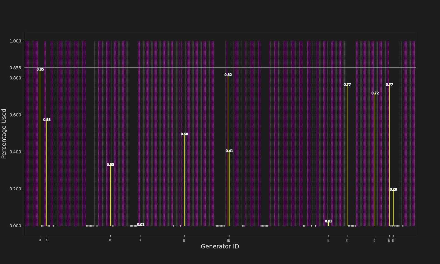
As discussed previously, to keep up with the increase in demand, a total of 198 new generators were installed. Despite all generators being assumed to be on and available to service the given load, 21 of the new generators were found to not be using any of their available capacity, while five were using some but not all of their available capacity, and 172 were using their full capacity. However, out of the total 297 generators considered, $241$ were observed to be using their full capacity, while $12$ were using some but not all of their available capacity, and $44$ were not using any of their available capacity. These results are summarized in Table 2 below.
| All | Some | None |
| New Generators | ||
| 172 | 5 | 21 |
| All Generators | ||
| 241 | 12 | 44 |
Additionally, Figure 1 displays these findings, and further shows the percentage of generation output by each individual generator, $g$, and overall output percentage for all generating units available.
References
- Moulin, L., Poss, M., & Sagastizábal, C. (2010). Transmission Expansion Planning with Re-Design. Energy Systems, 1, 113–139. https://doi.org/10.1007/s12667-010-0010-9
- Mutlu, S., & Şenyiğit, E. (2021). Literature review of transmission expansion planning problem test systems: detailed analysis of IEEE-24. Electric Power Systems Research, 201, 107543. https://doi.org/https://doi.org/10.1016/j.epsr.2021.107543
- Grigg, C., Wong, P., Albrecht, P., Allan, R., Bhavaraju, M., Billinton, R., Chen, Q., Fong, C., Haddad, S., Kuruganty, S., Li, W., Mukerji, R., Patton, D., Rau, N., Reppen, D., Schneider, A., Shahidehpour, M., & Singh, C. (1999). The IEEE Reliability Test System-1996. A report prepared by the Reliability Test System Task Force of the Application of Probability Methods Subcommittee. IEEE Transactions on Power Systems, 14(3), 1010–1020. https://doi.org/10.1109/59.780914